
Overview
Buying a home is a big decision, and negotiating the final sales price is a central part of that decision. If your offer is too low, it might be ignored. If it is too high, you end up spending more than required. Obviously, both these scenarios should be avoided, so how do you know if there is room to negotiate? One way is to not only estimate the expected price of a potential home relative to the asking price but also to quantify the certainty surrounding that estimate. Popular real-estate websites, such as Redfin or Zillow, provide the first part of this equation but do not provide any indication as to the certainty surrounding their estimate of a home’s value. A negotiable price would have the following two characteristics:
- An estimated value below the asking price
- A high level of confidence in the accuracy of the estimated value
In this post, I’ll cover how to generate insights on both fronts using the Boston Housing Dataset. However, before diving into the code, let’s briefly review some key concepts.
Confidence & Prediction Intervals
These two terms are often used interchangeably but they are quite different. In this case, we want to estimate a home’s sales price as a function of how many rooms are in the house. Confidence intervals capture uncertainty around a parameter estimate (e.g., the average increase in price for each additional room). If we were to repeatedly take samples of houses, measure their sales price and number of rooms, and calculate a different regression equation for each sample, then 95% of the confidence intervals generated from each regression should contain the true parameter (i.e., the increase in a home’s value resulting from each additional room).
Prediction intervals take the uncertainty of parameter estimates into account as well. But they also consider the uncertainty around trying to predict the value of an unseen, single observation (variability of individual observations around the parameter). Therefore, prediction intervals are always wider than confidence intervals – because we are considering more sources of uncertainty. When purchasing a home, we aren’t particularly interested in the average price of all homes with, say, eight rooms. What we want to know is the price for that eight-room, English Tudor Revival home with the old Oak tree in the front yard and 1980s style Jacuzzi in the backyard that’s for sale up the street. To answer that question, you’ll need to use a prediction interval.
With these differences in mind, let’s see how prediction intervals are used in practice. Imagine you are buying a home. You have actual historical sales data associated with various features of a home, such as the number rooms or commute time to major employment centers. You have the same data for homes you want to purchase, but instead of a sales price, you have an asking price. To recreate this situation, we’ll do a 70-30 split to create our training and test sets, respectively, using the Boston Housing dataset. We’ll implement cross-validation on the training set to get an idea of how well our prediction interval methodology will perform on new, unseen data. Finally, we’ll identify all the homes where an offer below the listing price has a high chance of being accepted. Let’s get started and pull all the data we’ll need into R.
libs = c('randomForest', 'dplyr', 'data.table',
         'knitr', 'ggplot2', 'kableExtra',
         'car', 'forcats', 'lazyeval',
         'broom', 'VSURF','quantregForest'
         )

lapply(libs, require, character.only = TRUE)

housing_data = fread("https://archive.ics.uci.edu/ml/machine-learning-databases/housing/housing.data",
                      data.table = FALSE)

names(housing_data) = c('crim', 'zn', 'indus',
                       'chas', 'nox', 'rm', 'age',
                       'dis', 'rad', 'tax', 'ptratio',
                       'b', 'lstat', 'sales_price')
# covert outcome variable to 100K increments
housing_data$sales_price = housing_data$sales_price * 10e3
set.seed(123)
pct_train = 0.70

train_indices = sample.int(n = nrow(housing_data),
                           size = floor(pct_train * nrow(housing_data)),
                           replace = FALSE)

train_df = housing_data[train_indices,]
test_df = housing_data[-train_indices,] %>%
          dplyr::rename(asking_price = sales_price)
As always, it’s a good idea to check out a few rows in the data.
| crim | zn | indus | chas | nox | rm | age | dis | rad | tax | ptratio | b | lstat | sales_price | |
|---|---|---|---|---|---|---|---|---|---|---|---|---|---|---|
| 146 | 2.37934 | 0 | 19.58 | 0 | 0.871 | 6.130 | 100.0 | 1.4191 | 5 | 403 | 14.7 | 172.91 | 27.80 | 138000 |
| 399 | 38.35180 | 0 | 18.10 | 0 | 0.693 | 5.453 | 100.0 | 1.4896 | 24 | 666 | 20.2 | 396.90 | 30.59 | 50000 |
| 207 | 0.22969 | 0 | 10.59 | 0 | 0.489 | 6.326 | 52.5 | 4.3549 | 4 | 277 | 18.6 | 394.87 | 10.97 | 244000 |
| 445 | 12.80230 | 0 | 18.10 | 0 | 0.740 | 5.854 | 96.6 | 1.8956 | 24 | 666 | 20.2 | 240.52 | 23.79 | 108000 |
| 473 | 3.56868 | 0 | 18.10 | 0 | 0.580 | 6.437 | 75.0 | 2.8965 | 24 | 666 | 20.2 | 393.37 | 14.36 | 232000 |
| 23 | 1.23247 | 0 | 8.14 | 0 | 0.538 | 6.142 | 91.7 | 3.9769 | 4 | 307 | 21.0 | 396.90 | 18.72 | 152000 |
| 265 | 0.55007 | 20 | 3.97 | 0 | 0.647 | 7.206 | 91.6 | 1.9301 | 5 | 264 | 13.0 | 387.89 | 8.10 | 365000 |
| 446 | 10.67180 | 0 | 18.10 | 0 | 0.740 | 6.459 | 94.8 | 1.9879 | 24 | 666 | 20.2 | 43.06 | 23.98 | 118000 |
| 275 | 0.05644 | 40 | 6.41 | 1 | 0.447 | 6.758 | 32.9 | 4.0776 | 4 | 254 | 17.6 | 396.90 | 3.53 | 324000 |
| 227 | 0.38214 | 0 | 6.20 | 0 | 0.504 | 8.040 | 86.5 | 3.2157 | 8 | 307 | 17.4 | 387.38 | 3.13 | 376000 |
Great success! Each of the fields represents some attribute of the home For example, rm is the number of rooms in the house, and crim is the per capita crime rate per town (see here for more detail). We are now ready to build a model, and the first step is to understand which features are essential to our prediction accuracy. We’ll leverage the VSURF package, or Variable Selection Using Random Forest, to do variable selection, ensuring that only features that matter enter into the model. This is achieved in a stepwise fashion, where the Out of Bag (OOB) errors are compared between models that include/exclude one variable. If a big reduction in the average OOB error occurs when a variable is included, then we assume that the variable is important.
set.seed(123)
vsurf_fit = VSURF(x = train_df[,1:13],
            y = train_df[,14],
            parallel = TRUE,
            ncores = 8)
The following four variables contributed significantly to the selling price of a home in Boston:
- lstat - % lower status of the population
- rm - number of rooms
- nox - nitric oxides concentration (not sure if this is good or bad)
- dis - weighted distance to five Boston employment centers
Let’s reduce our training set to only include these four features.
train_df = train_df[c(names(train_df)[vsurf_fit$varselect.pred],
                       'sales_price')]
x_var = setdiff(names(train_df), 'sales_price')
Now that we have our new, slim data set, we’ll move on to the modeling part. In this case, we’ll use a technique called Quantile Regression or QR. For those unfamiliar, QR works by differentially weighting errors during the model fitting process. It captures the relationship between our inputs and a specific quantile (i.e., percentile) of our output. For example, if the goal is to understand the relationship between X and Y at the 90th percentile of Y, 10% of the errors should be positive and 90% negative to minimize our loss function (e.g., MAE, MSE). This is especially useful for creating prediction intervals, while also providing a point estimate, in this case, the median (i.e., the 50th percentile). Additionally, it is agnostic to the statistical method being used; multiple regression is the most common form of quantile regression, but GBM, Random Forest, which is what will be used here, and even Neural Networks can be used to do QR.
With that in mind, let’s move on to the actual modeling part. First, we’ll determine how well we can explain a home’s sale price via the Mean Absolute Error (MAE). Second, we’ll validate our prediction intervals. An 80% prediction interval will be used, so at least 80% of observations should fall within the bounds of an interval – a metric referred to as coverage or tolerance. We’ll test both metrics via 5-fold cross-validation.
set.seed(123)
# add row index
train_df$row_index = 1:nrow(train_df)
# shuffle rows to randomized input order
train_df = train_df[sample(nrow(train_df)),]
# specify N folds
n_fold = 5
start_index = 1
end_index = floor(nrow(train_df)/n_fold)
increment = end_index
cv_df = data.frame(NULL)
for(i in 1:n_fold){
  temp_train_df = train_df %>%
                  filter(!(row_index %in% start_index:end_index)) %>%
                  select(-row_index)

  temp_validation_df = train_df %>%
                  filter(row_index %in% start_index:end_index) %>%
                  select(-row_index)

  cv_pred = tidy(
                  predict(quantregForest(x = temp_train_df[,1:(dim(temp_train_df)[2] - 1)],
                                         y = temp_train_df[,dim(temp_train_df)[2]],
                                         ntree = 500
                                        ),
                          temp_validation_df,
                          what = c(0.1, 0.5, 0.9)
                          )
                  ) %>%
             mutate(sales_price = temp_validation_df$sales_price) %>%
             rename(lwr = quantile..0.1,
                    upr = quantile..0.9,
                    predicted_price = quantile..0.5
                    ) %>%
             mutate(residual = sales_price - predicted_price,
                    coverage = ifelse(sales_price > lwr & sales_price < upr, 1, 0)
                    )
  cv_df = bind_rows(cv_df,
                    data.frame(mean_abs_err = mean(abs(cv_pred$residual)),
                               coverage = sum(cv_pred$coverage)/nrow(cv_pred) * 100,
                               fold = i
                              )
                    )
  start_index = end_index
  end_index = end_index + increment
  if(end_index > nrow(train_df)){
    break
  }
}| mean_abs_err | coverage | fold |
|---|---|---|
| 21192.86 | 87.14286 | 1 |
| 28345.07 | 84.50704 | 2 |
| 25563.38 | 83.09859 | 3 |
| 23119.72 | 90.14085 | 4 |
| 25654.93 | 81.69014 | 5 |
Overall the model and prediction intervals performed well, at least well enough to the point where I’d feel comfortable negotiating based on the output. Let’s put our new-found knowledge to work! First, to make this example more realistic, we’ll apply a few constraints. For example, I want a house with at least six rooms, within an average distance of four miles to all major working areas (because sitting in traffic is no fun), and I don’t want to spend any more than 300K. Let’s filter the test data set to only include homes that meet these criteria.
rm_threshold = 6
dis_threshold = 4
price_threshold = 300000
test_df = test_df %>%
          select(c(x_var, 'asking_price')) %>%
          filter(rm >= rm_threshold &
                 dis <= dis_threshold &
                 asking_price <= price_threshold
                   )
A total of 48 homes remain. Of these homes, which could we negotiate the sale price? Let’s examine the output from our final model and visualize where the opportunities exist.
qrf_fit = quantregForest(x=train_df[,1:4],
                         y = train_df[,5],
                         ntree = 1000)

qrf_quantile = predict(qrf_fit,
                        test_df,
                        what=c(0.1, 0.5, 0.9)) %>%
                data.frame() %>%
                rename(predicted_price = quantile..0.5,
                       lwr = quantile..0.1,
                       upr = quantile..0.9) %>%
                mutate(asking_price = test_df$asking_price) %>%
                mutate(coverage = ifelse(asking_price <= upr & asking_price >= lwr,
                                         1,
                                         0),
                       `PI Range` = upr - lwr,
                       residual = asking_price - predicted_price
                       ) %>%
                mutate(Opportunity = ifelse(residual < 0,
                                            "underpriced",
                                            "overpriced")) %>%
                filter(`PI Range` <= 90000)


qrf_plot_input = qrf_quantile %>%
  mutate(asking_price = asking_price/1e3,
         predicted_price = predicted_price/1e3,
         `PI Range` = `PI Range`/1e3,
         lwr = lwr/1e3,
         upr = upr/1e3
         )
# custom plotting theme
my_plot_theme = function(){
font_family = "Helvetica"
font_face = "bold"
return(theme(
axis.text.x = element_text(size = 18, face = font_face, family = font_family),
axis.text.y = element_text(size = 18, face = font_face, family = font_family),
axis.title.x = element_text(size = 20, face = font_face, family = font_family),
axis.title.y = element_text(size = 20, face = font_face, family = font_family),
strip.text.y = element_text(size = 18, face = font_face, family = font_family),
plot.title = element_text(size = 18, face = font_face, family = font_family),
legend.position = "top",
legend.title = element_text(size = 16,
face = font_face,
family = font_family),
legend.text = element_text(size = 14,
face = font_face,
family = font_family)
))
}ggplot(qrf_plot_input, aes(x = asking_price,
y = predicted_price,
color = Opportunity)) +
theme_bw() +
geom_point(aes(size = `PI Range`)) +
geom_errorbar(aes(ymin = lwr, ymax = upr)) +
geom_abline(intercept = 0, slope = 1,
color = "black", size = 2,
linetype = "solid",
alpha = 0.5
) +
xlab("Asking Price (K)") + ylab("Predicted Price (K)") +
my_plot_theme() +
xlim(0, price_threshold/1e3 + 30) + ylim(0, price_threshold/1e3 + 30) +
annotate("segment",
x = 260,
xend = 285,
y = 200,
yend = 228,
colour = "black",
size = 2,
arrow = arrow(),
alpha = 0.6
)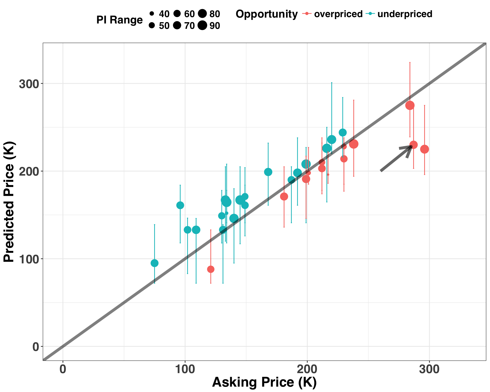
Each point represents a home. All points below the diagonal line are overpriced homes (i.e., the asking price is above the predicted price), while those above the diagonal line are underpriced. Each of the points is sized according to the width of its prediction interval, such that smaller points have narrower intervals. The arrow identifies a potential home that we should feel comfortable negotiating on price because it not only is overpriced but also has a relatively narrow prediction interval. When both features are present, making an offer for less than the asking price should result in an acceptance more frequently than the points above of the line or those with wider prediction intervals. This is information we can use to decide when to make a purchase, continue negotiating, or simply walk away from the house.
Concluding Remarks
This post outlined a framework for identifying opportunities where an offer lower than the asking price would likely be accepted when purchasing a home. However, this framework could be used in any decision-making context where uncertainty is a major factor in choosing a course of action. For example, imagine we were predicting demand for a new product instead of home prices. If our demand forecast was much larger than production numbers, and the accompanying prediction interval was small, then we could recommend an increase in production numbers to avoid lost sales. I’d love to hear about frameworks/techniques that you use to deal with these types of issues, so please feel free to chime in below!