
Overview
Trend detection is way to anticipate where something will go in the future. The logic underlying the inference is simple: Are there patterns of activity that precede an upward or downward trend? For example, a fashion trend might start in a big city like New York, London, or Paris. The emergence of the trend might then occur at a later date in smaller nearby cities. Thus, if you were charged with anticipating future demand for the trending product, you could use the early signal from the big cities to anticipate demand in the smaller cities. This information could inform everything from design to demand planning (i.e., getting the right amount of product in the right place). This is often referred to as a leading indicator.
For this approach to be effective, there has to be a “common way” in which a something trends. Maybe it’s a gradual increase over the first five days, followed by a rapid increase over the next 10 days. Or maybe you just need the first three days to make an accurate prediction of a positive trend when the change in demand is very rapid. There are many ways in which something can trend, but the pattern of demand, tweets, views, purchases, likes, etc. for a positive trend has to be different from a negative or flat trend.
This post outlines one approach to separate the signatures associated with different types of trends. We’ll use stock data from Fortune 500 companies as our analytical dataset to predict if a stock’s price will trend positively based on its closing price over the first 30 days in Jan/Feb of 2015? Before jumping into the example, though, I’ll briefly introduce the technique with a smaller dataset.
Non-Parametric Trend Detection
We’ll use a K-Nearest-Neighbor (KNN) approach for classifying where a stock’s price trend in the future (i.e., up or flat/down). KNN is non-parametric, which means we don’t make any assumptions about our data. There is also no ‘model’; we simply let the data make the classification or prediction. Without generalizing too much, I’ve liked KNN when my feature set is small and consists mostly of continuous variables. It is easy to explain and surprisingly effective relative to more complicated, parametric models. All we have to do is find the right “K”, which is the number of neighbors we use to make our prediction/classification. “K” is determined through cross-validation, where we try several values and see which gives the best results.
So how do we determine our neighbors? There are many distance metrics used to define “similarity”, the most common being Euclidean Distance. However, the main drawback to this approach is that it cannot account for forward or backward shifts between series, which is an issue when dealing with sequential data. Thus we’ll use Dynamic Time Warping, which can account for temporary shifts, leads, or lags.
We’ll use 10 fictitious stocks in our initial example. Five will trend positively after their first 50 days while the remaining five will trend negatively over the same time period. These stocks will serve as our “training set”. We’ll then take a new stock for which we only have the first 50 days and classify it as either a “positive” or “negative” trending stock. This prediction is where we think the stock will go relative to its position at day 50.
Let’s first generate the initial 50 days for our 10 stocks.
libs = c('BatchGetSymbols', 'rvest', 'Kendall',
         'dplyr','openair', 'broom',
         'MarketMatching', 'ggplot2', 'knitr',
         'ggforce', 'rvest', 'xml2',
         'janitor'
         )
lapply(libs, require, character.only = TRUE)
set.seed(123)
pre_date_range = seq.Date(as.Date("2016-01-01"),
                          by = "day",
                          length = 100)
pre_period = 50
trend_patterns = data.frame()
for(i in 1:5){
  # generate pattern for stocks that trend negatively from days 51-100
  neg_trend_pre = cos(seq(0, 10, 0.1))[1:pre_period] + rnorm(pre_period, 0, 0.7)
  trend_patterns = bind_rows(trend_patterns,
                         data.frame(date = pre_date_range[1:pre_period],
                                    value = neg_trend_pre,
                                    class = paste0('negative_', i)))

  # generate pattern for stocks that trend positively from days 51-100
  pos_trend_pre = cos(seq(0, 10, 0.1))[(pre_period + 1):100] + rnorm(pre_period, 0, 0.7)
  trend_patterns = bind_rows(trend_patterns,
                        data.frame(date = pre_date_range[1:pre_period],
                                          value = pos_trend_pre,
                                          class = paste0("positive_", i)))
}
Now let’s add in our positive and negative trends.
generate_trend = function(trend_length, increment, sd, base_value){
    trend_vector = c()
    for(j in 1:trend_length){
        trend_vector = c(trend_vector, rnorm(1,
                                             base_value,
                                             sd = sd))
        base_value = base_value + increment
    }
    return(trend_vector)
}

increment = 0.03
standard_dev = 0.08
trend_patterns_future = data.frame(NULL)
for(temp_trend in unique(trend_patterns$class)){
    temp_ts = trend_patterns %>%
              filter(class == temp_trend)
    # extend date 50 days forward
    future_dates = pre_date_range[51:length(pre_date_range)]
    base_value = temp_ts$value[length(temp_ts$value)]
    future_trend = generate_trend(length(future_dates),
                                  increment,
                                  standard_dev,
                                  base_value)
    if(strsplit(temp_trend, "_")[[1]][1] == 'negative'){
        future_trend = future_trend * -1
        }
    trend_patterns_future = bind_rows(trend_patterns_future,
                                      data.frame(date = future_dates,
                                                 value = future_trend,
                                                 class = temp_trend)
                                  )
}

trend_patterns_ex = bind_rows(trend_patterns,
                              trend_patterns_future) %>%
                              arrange(class, date)
And finally, we’ll set up our plotting function and plot the five positive and five negative trends. Additionally, we’ll look at the first 50 days to see if there is a pattern associated with positive/negative trends. The gray shaded area indicates the point at which we make our prediction regarding where we think the stock will go.
my_plot_theme = function(){
    font_family = "Helvetica"
    font_face = "bold"
    return(theme(
    axis.text.x = element_text(size = 18, face = font_face, family = font_family),
    axis.text.y = element_text(size = 18, face = font_face, family = font_family),
    axis.title.x = element_text(size = 20, face = font_face, family = font_family),
    axis.title.y = element_text(size = 20, face = font_face, family = font_family),
    strip.text.y = element_text(size = 18, face = font_face, family = font_family),
    plot.title = element_text(size = 18, face = font_face, family = font_family),
    legend.position = "top",
    legend.title = element_text(size = 16,
    face = font_face,
    family = font_family),
    legend.text = element_text(size = 14,
    face = font_face,
    family = font_family)
))
}
# plotting colors
plot_colors = c("#33FFFB","#33D6FF",
"#33BDFF","#3388FF",
"#33EAFF","#FF3371",
"#FF335C","#FF334C",
"#FF4833","#FF5833")
ggplot(trend_patterns_ex, aes(x = date, y = value, color = class)) +
geom_point(alpha = 0.2) + stat_smooth(se = FALSE) +
scale_color_manual(values = plot_colors) +
theme_bw() +
my_plot_theme() +
ylab("Stock Price") + xlab("Date") +
facet_zoom(x = date %in% pre_date_range[1:pre_period])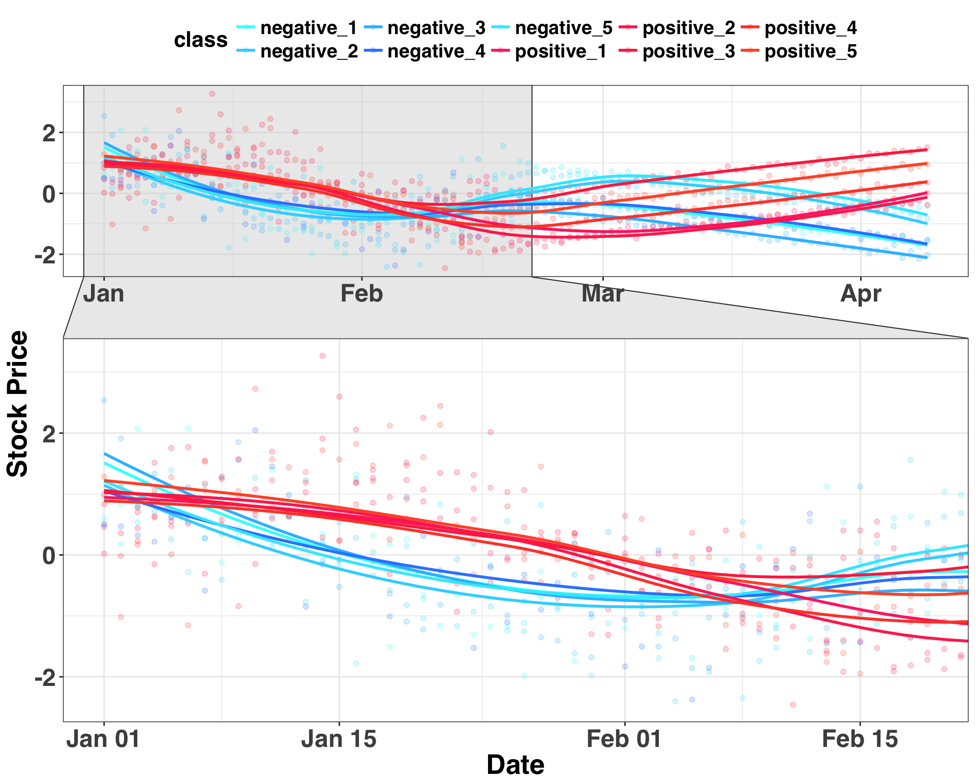
In this case, stocks that initially go up, drift down, then flatten out all trend positively. In contrast, stocks that decline and then increase from days 30-50 trend downward from days 51-100. Thus, there is a common pattern that precedes a sustained increase or decrease in price. Based on this information, let’s introduce our new stock – the “target trend” – that we only have pricing information for days 1-50.
sample_trend_pre = bind_rows(data.frame(date = pre_date_range[1:pre_period],
                                        value = cos(seq(0, 10, 0.1))[(pre_period + 1):100] + rnorm(pre_period, 0, 0.7),
                                        class = "target_trend"),
                             data.frame(date = rep(NA, pre_period),
                                        value = rep(NA, pre_period),
                                        class = "target_trend")
                             )
trend_patterns_ex = bind_rows(sample_trend_pre,
                              trend_patterns_ex)
ggplot(trend_patterns_ex, aes(x = date, y = value, color = class)) +
geom_point(alpha = 0.1) + geom_line(stat = "smooth",
method = "gam",
formula = y ~ s(x),
size = 2,
alpha = 0.2
) +
scale_color_manual(values = c("black", plot_colors)) +
theme_bw() +
my_plot_theme() +
stat_smooth(data = sample_trend_pre,
aes(x = date, y = value),
color = "black",
se = FALSE,
size = 3,
lty = 4) +
theme(legend.position = "none") +
ylab("Stock Price") +
facet_zoom(x = date %in% pre_date_range[1:pre_period])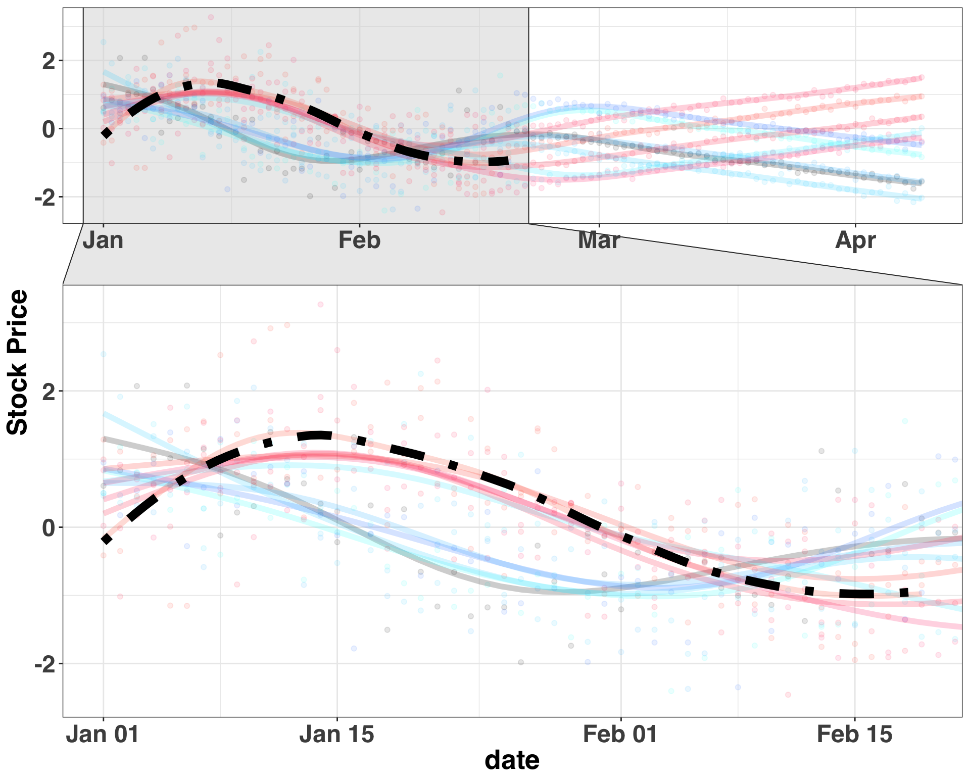
Let’s filter our dataset to days 1-50 and see how many of the nearest neighbors for our target trend are positive/negative. In this case K is set to 5.
trend_patterns_test_time = trend_patterns_ex %>%
                           filter(date <= as.Date("2016-02-19")) %>%
                           mutate(class = as.character(class))

trend_pattern_matches = best_matches(data = trend_patterns_test_time,
                                     id_variable = "class",
                                     date_variable = "date",
                                     matching_variable = "value",
                                     parallel = TRUE,
                                     warping_limit = 3,
                                     matches = 5,
                                     start_match_period = min(trend_patterns_test_time$date),
                                     end_match_period = max(trend_patterns_test_time$date)
)

best_matches = trend_pattern_matches$BestMatches %>%
filter(class == 'target_trend')| class | BestControl | RelativeDistance | Correlation | Length | rank | MatchingStartDate | MatchingEndDate |
|---|---|---|---|---|---|---|---|
| target_trend | positive_2 | 3.234196 | 0.6145986 | 50 | 1 | 2016-01-01 | 2016-02-19 |
| target_trend | positive_4 | 3.375498 | 0.5205792 | 50 | 2 | 2016-01-01 | 2016-02-19 |
| target_trend | positive_3 | 3.394093 | 0.5089169 | 50 | 3 | 2016-01-01 | 2016-02-19 |
| target_trend | positive_1 | 3.408172 | 0.5831835 | 50 | 4 | 2016-01-01 | 2016-02-19 |
| target_trend | positive_5 | 3.453815 | 0.4916183 | 50 | 5 | 2016-01-01 | 2016-02-19 |
Let’s focus on the BestControl field. All five of the most similar time-series to our target time-series have a positive label. Thus we would predict that our target time-series will trend positively from days 51-100, based on its pattern from days 1-50. If all five of our best matches were stocks that negatively trended, then we would make the opposite prediction. I told you this method is simple (and effective)! However, let’s see if how we feel the same way after working with real-world stock data, introduced in the next section.
Predicting Stocks
We are trying to answer the following question:
- Is there a pattern of daily closing prices that comes before a ~90-day increase in the price of a stock?
For example, maybe a small increase in the first 60 days is often followed by a big 60-day upward climb. Or maybe stocks that gradually dip for a period of 60 days are more likely to rebound over the subsequent 60 days. In essence, are there a collection of 60-day patterns that come before an upward trend in a stock’s price? Trying to formalize such patterns with a set of parameters is difficult, given the variety of patterns that could be associated with a positive trend. This is why we are using the approach outlined above and letting the data decide.
We’ll begin by scraping the names of all Fortune 500 companies from Wikipedia, and then pull the actual closing prices for each company via the BatchGetSymbols package. This will take a few minutes.
url = "https://en.wikipedia.org/wiki/List_of_S%26P_500_companies"

# collect fortunue 500 stock symbols
stock_names = url %>%
       read_html() %>%
       html_nodes(xpath='//*[@id="mw-content-text"]/div/table[1]') %>%
       html_table() %>%
       pull(Ticker.symbol)

train_period_begin = as.Date("2015-01-01")
train_period_end = max(seq(train_period_begin, by = "day", length.out = 200))
# collect actual closing prices for stocks
stock_price = BatchGetSymbols(tickers = stock_names,
                              first.date = train_period_begin,
                              last.date = train_period_end
                              )$df.tickers %>%
              clean_names() %>%
select(ref_date, ticker, price_close)| ticker | ref_date | price_close |
|---|---|---|
| MMM | 2015-01-02 | 164.06 |
| MMM | 2015-01-05 | 160.36 |
| MMM | 2015-01-06 | 158.65 |
| MMM | 2015-01-07 | 159.80 |
| MMM | 2015-01-08 | 163.63 |
| MMM | 2015-01-09 | 161.62 |
| MMM | 2015-01-12 | 160.74 |
| MMM | 2015-01-13 | 160.62 |
| MMM | 2015-01-14 | 159.84 |
| MMM | 2015-01-15 | 159.66 |
Data looks ready to go! Let’s select the stocks that will comprise our training/test sets. We’ll do a 90⁄10 split. Note that the test stocks will be used a little later.
set.seed(123)
n_days_train = 60
n_day_outcome = 60
pct_stocks_in_test = 0.1
# select stocks that will be in the training and test sets
test_stocks = sample(stock_names,
                     size = floor(length(unique(stock_price$ticker)) * pct_stocks_in_test),
                     replace = FALSE)

train_stocks = setdiff(stock_price$ticker, test_stocks)
# select first 30 days of 2015 as feature set
input_dates = unique(stock_price$ref_date)[1:n_days_train]
# select next 90 days as trend outcome
trend_dates = setdiff(unique(stock_price$ref_date), input_dates)[1:n_day_outcome]
stocks_train = stock_price %>%
               filter(ticker %in% train_stocks) %>%
               mutate(label = ifelse(ref_date %in% input_dates,
                                     "input_dates",
                                     "trend_dates"))
Now that we have our data and it’s all cleaned up, let’s discuss how we’ll determine the labels for our “positive” and “flat|negative” time series.
Defining a Trend
We could plot out every time series and label them by hand but ain’t nobody got time for that. Instead, we’ll use two automated approaches:
- Linear Regression (LR)
- Mann-Kendall test (MK)
Labels will be generated based on the trend observed from days 60-120 and will be either positive, negative, or neutral. We are interested in whether the coefficient for this index is significant as well as its overall direction. For example, if a stock exhibits a significant positive trend, then it will be labeled positive; if a stock exhibits random variation, then it will be labeled neutral. LR takes the average slope, while the MK approach takes the median slope. Note that we might be violating the assumption that our data points are uncorrelated with one another. There are ways around this (e.g., block bootstrapping), but for the sake of simplicity, we’ll assume an absence of serial correlation. Let’s run both tests and gather the results.
# use mann-kendall to determine class
mk_class = stocks_train %>%
              filter(label == "trend_dates") %>%
              group_by(ticker) %>%
              do(trend_data = MannKendall(ts(.$price_close))) %>%
              data.frame()

mk_class$tau = unlist(lapply(mk_class$trend_data,
                                function(x) x[[1]][1]))
mk_class$p_value = unlist(lapply(mk_class$trend_data,
                                    function(x) x[[2]][1]))

ELSE = TRUE
mk_class = mk_class %>%
           select(ticker, tau, p_value) %>%
           mutate(trend_class_mk = case_when(tau > 0 & p_value < 0.01 ~ "positive",
                                   tau < 0 & p_value < 0.01 ~ "negative",
                                   ELSE ~ "neutral"
                                    )) %>%
           select(ticker, trend_class_mk)

# use linear regression to determine class
lm_class = stocks_train %>%
  filter(label == "trend_dates") %>%
  group_by(ticker) %>%
  mutate(day_index = row_number()) %>%
  do(tidy(lm(price_close ~ day_index, data = .))) %>%
  filter(term == 'day_index') %>%
  mutate(trend_class_lm = case_when(p.value < 0.01 & estimate > 0 ~ "positive",
                                    p.value < 0.01 & estimate < 0 ~ "negative",
                                    ELSE ~ "neutral"
                                    )) %>%
  select(ticker, trend_class_lm)

trend_class = inner_join(mk_class,
                         lm_class,
on = "ticker")| ticker | trend_class_mk | trend_class_lm |
|---|---|---|
| A | negative | negative |
| AAL | negative | negative |
| AAP | positive | positive |
| AAPL | neutral | neutral |
| ABBV | positive | positive |
| ABC | negative | negative |
| ABT | positive | positive |
| ACN | positive | positive |
| ADBE | positive | positive |
| ADI | neutral | neutral |
The two methods produced the same classification for most of the stocks. However, let’s examine a few cases where they differ.
stocks_train %>%
filter(ticker == 'ADI' & label == 'trend_dates') %>%
mutate(ref_date = as.Date(ref_date)) %>%
ggplot(aes(x = ref_date, y = price_close)) +
      geom_point(size = 2, color = "black") +
      geom_line(size = 2, color = "black") +
      theme_bw() +
      my_plot_theme() +
      ylab("Closing Price") +
      xlab("Date")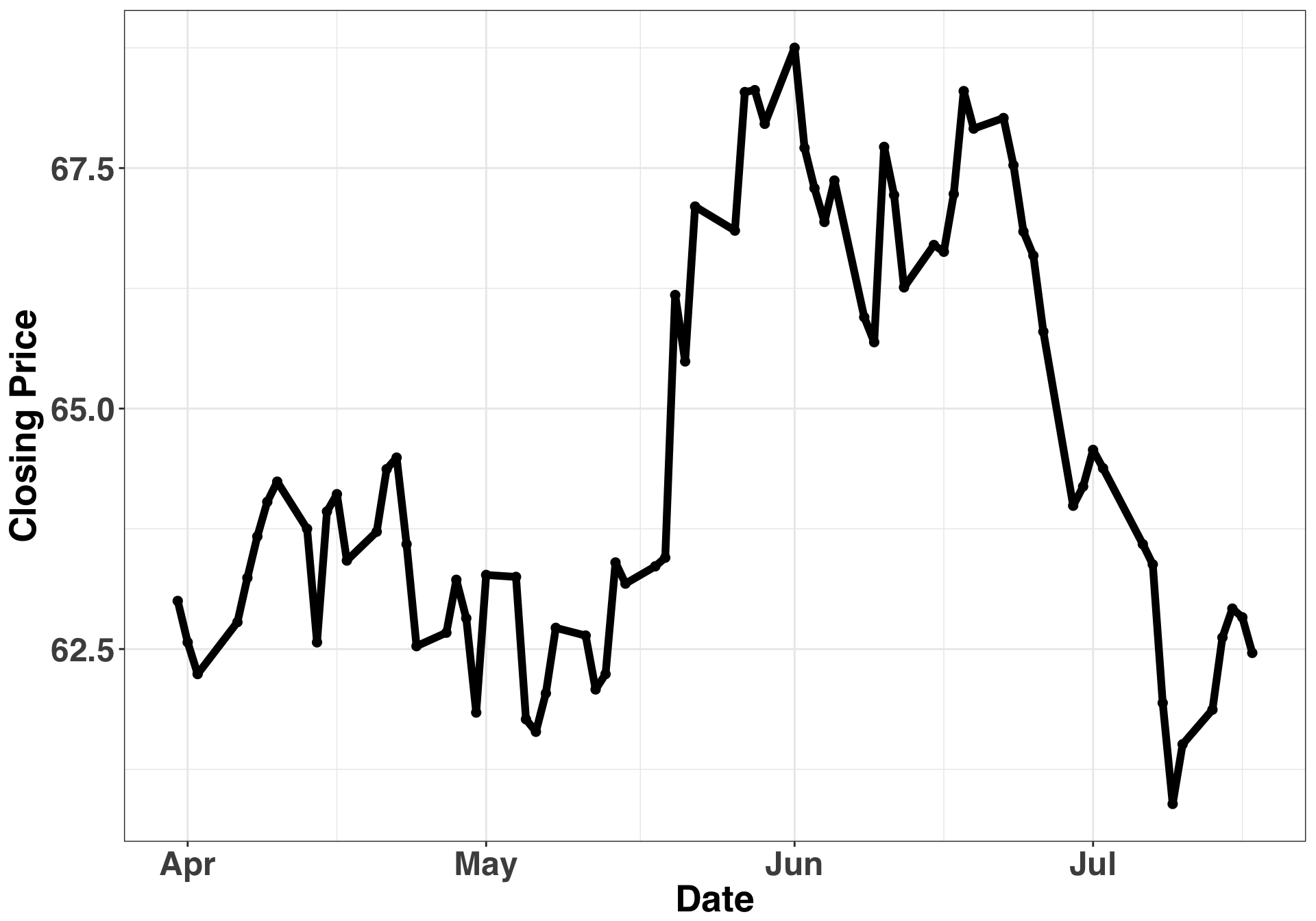
The price for this stock goes up but then trends downward. The LR indicates a positive trend while the MK test indicates a neutral trend. The LR is taking the average, and the average is positive overall, given that the stock showed big gains in June and July. In contrast, the MK tests whether there is a monotonically increasing or decreasing trend over time. It is considering the ratio of positive and negative differences across time. Since we went up and then back down, there will be a similar number of positive/negative differences, hence the neutral classification.
Let’s consider a separate example.
stocks_train %>%
filter(ticker == 'NI' & label == 'trend_dates') %>%
mutate(ref_date = as.Date(ref_date)) %>%
ggplot(aes(x = ref_date, y = price_close)) +
      geom_point(size = 2, color = "black") +
      geom_line(size = 2, color = "black") +
      theme_bw() +
      my_plot_theme() +
      ylab("Closing Price") +
      xlab("Date")
This time series produced the exact oppositive pattern: The MK test classified the trend as neutral, while the LR produced a negative classification. The stock trended slightly upward for most of the time-period and then crashed the last few days in July. Those final few points have a lot of leverage on the coefficient in the linear model, while the MK test is relatively unaffected. In this case, I’d say it’s a negatively trending stock, but arguments for either classification could be made.
Stocks such as these are why we are evaluating two separate viewpoints. We want to ensure that the trend is somewhat definitive. If there is disagreement amongst the methods, we are going to assign a stock the “neutral” label. In a more formal analytical setting, we would spend more time testing whether this labeling approach is valid. However, for the sake of illustration, we’re going to use a simple, heuristic-based approach, such that any classification disagreements amongst the two methods will result in a neutral classification. Let’s update all of the instances where a disagreement occurred, and then filter out all of the neutral cases.
trend_class = trend_class %>%
              mutate(trend_class = ifelse(trend_class_mk != trend_class_lm,
                                         "neutral",
                                         trend_class_mk)) %>%
              select(ticker, trend_class) %>%
              filter(trend_class != "neutral")
Finally, let’s examine the distribution of our classes.
print(table(trend_class$trend_class))
print("----------------------------------")
print(paste0("PERCENT OF STOCKS POSITIVE: ",
      round(table(trend_class$trend_class)[[2]]/nrow(trend_class) * 100, 0),
      "%")
      )
##
## negative positive
## 195 150
## [1] "----------------------------------"
## [1] "PERCENT OF STOCKS POSITIVE: 43%"There are more time series in negative class relative to the positive class. This isn’t a huge imbalance, but it might skew our classifications toward the negative class, as there are simply more series to match on. Let’s downsample our negative stocks so we have an equal number of positive and negative classes in the training set.
set.seed(123)
trend_class = trend_class %>%
              filter(trend_class == "negative") %>%
              sample_n(trend_class %>%
                       filter(trend_class == "positive") %>%
                       nrow()
                         ) %>%
              bind_rows(trend_class %>%
                        filter(trend_class == "positive"))

print(table(trend_class$trend_class))
##
## negative positive
## 152 152print("----------------------------------")## [1] "----------------------------------"print(paste0("PERCENT OF STOCKS POSITIVE: ",round(table(trend_class$trend_class)[[2]]/nrow(trend_class) * 100, 0), "%"))## [1] "PERCENT OF STOCKS POSITIVE: 50%"##
## negative positive
## 150 150
## [1] "----------------------------------"
## [1] "PERCENT OF STOCKS POSITIVE: 50%"Perfect. Now we have even numbers and are ready to test out the trend detector.
Trend Detection Performance
Now that we’ve assigned a label to each of the stocks in our training set, we’ll download the closing prices for the test stocks, which are from the following year during the same time period (i.e., Jan/Feb 2016).
test_period_begin = as.Date("2016-01-01")
test_period_end = max(seq(test_period_begin,
                          by = "day",
                          length.out = 200))

stocks_test = BatchGetSymbols(tickers = test_stocks,
                              first.date = test_period_begin,
                              last.date = test_period_end)$df.tickers %>%
                   clean_names() %>%
                   select(ref_date, ticker, price_close)
##
## Running BatchGetSymbols for:
## tickers = DLPH, REGN, FTV, TWX, VRSN, AGN, JBHT, TJX, KMI, HRS, VZ, HAL, NEM, LH, AIV, TXT, CMS, ALGN, DPS, URI, SYF, NWSA, MET, WMT, MSFT, NI, IQV, LEG, CSX, BDX, UA, SRCL, MYL, PPL, AMG, HBI, PCAR, CERN, DVN, CMG, BK, FAST, FB, EW, VIAB, BHGE, CVX, GE, KO
## Downloading data for benchmark ticker
## Downloading Data for DLPH from yahoo (1|49) - Nice!
## Downloading Data for REGN from yahoo (2|49) - Got it!
## Downloading Data for FTV from yahoo (3|49) - OK!
## Downloading Data for TWX from yahoo (4|49) - Nice!
## Downloading Data for VRSN from yahoo (5|49) - Good job!
## Downloading Data for AGN from yahoo (6|49) - Got it!
## Downloading Data for JBHT from yahoo (7|49) - Good stuff!
## Downloading Data for TJX from yahoo (8|49) - Got it!
## Downloading Data for KMI from yahoo (9|49) - Good stuff!
## Downloading Data for HRS from yahoo (10|49) - Nice!
## Downloading Data for VZ from yahoo (11|49) - Good job!
## Downloading Data for HAL from yahoo (12|49) - Nice!
## Downloading Data for NEM from yahoo (13|49) - Nice!
## Downloading Data for LH from yahoo (14|49) - Good stuff!
## Downloading Data for AIV from yahoo (15|49) - Well done!
## Downloading Data for TXT from yahoo (16|49) - Got it!
## Downloading Data for CMS from yahoo (17|49) - Nice!
## Downloading Data for ALGN from yahoo (18|49) - Got it!
## Downloading Data for DPS from yahoo (19|49) - Good job!
## Downloading Data for URI from yahoo (20|49) - Got it!
## Downloading Data for SYF from yahoo (21|49) - Boa!
## Downloading Data for NWSA from yahoo (22|49) - Well done!
## Downloading Data for MET from yahoo (23|49) - Good job!
## Downloading Data for WMT from yahoo (24|49) - Good job!
## Downloading Data for MSFT from yahoo (25|49) - Nice!
## Downloading Data for NI from yahoo (26|49) - Good stuff!
## Downloading Data for IQV from yahoo (27|49) - Boa!
## Downloading Data for LEG from yahoo (28|49) - Good job!
## Downloading Data for CSX from yahoo (29|49) - Well done!
## Downloading Data for BDX from yahoo (30|49) - Nice!
## Downloading Data for UA from yahoo (31|49) - Good job!
## Downloading Data for SRCL from yahoo (32|49) - Got it!
## Downloading Data for MYL from yahoo (33|49) - Good job!
## Downloading Data for PPL from yahoo (34|49) - Good stuff!
## Downloading Data for AMG from yahoo (35|49) - Got it!
## Downloading Data for HBI from yahoo (36|49) - Good stuff!
## Downloading Data for PCAR from yahoo (37|49) - Boa!
## Downloading Data for CERN from yahoo (38|49) - Boa!
## Downloading Data for DVN from yahoo (39|49) - Got it!
## Downloading Data for CMG from yahoo (40|49) - Nice!
## Downloading Data for BK from yahoo (41|49) - Boa!
## Downloading Data for FAST from yahoo (42|49) - Good job!
## Downloading Data for FB from yahoo (43|49) - Boa!
## Downloading Data for EW from yahoo (44|49) - Good stuff!
## Downloading Data for VIAB from yahoo (45|49) - Nice!
## Downloading Data for BHGE from yahoo (46|49) - Good job!
## Downloading Data for CVX from yahoo (47|49) - Got it!
## Downloading Data for GE from yahoo (48|49) - Good job!
## Downloading Data for KO from yahoo (49|49) - Got it!Now let’s union our test and training datasets together. We’ll also change the time-stamps in our testing data set, despite the fact that our training data is from 2015 and our testing data is from 2016.
stocks_train_match = stocks_train %>%
  inner_join(trend_class) %>%
  filter(ref_date %in% input_dates)

stocks_test_match = stocks_test %>%
  filter(ref_date %in% unique(stocks_test$ref_date)[1:n_days_train]) %>%
  mutate(ref_date = rep(unique(stocks_train_match$ref_date),
                        length(unique(stocks_test$ticker)))) %>%
  mutate(label = 'test_dates',
         trend_class = 'unknown'
         )

matching_df = bind_rows(stocks_train_match,
                        stocks_test_match
                        ) %>%
              mutate(ref_date = as.Date(ref_date))
We are going to initially set K to 10. The reason why we’re using such a high number is that some of the test stocks will match with other test stocks. Obviously, these won’t have labels, so we only want to consider matches with training stocks. This section will take a few minutes to run.
max_matches = 10
best_match_df = best_matches(data = matching_df,
                             id_variable = "ticker",
                             date_variable = "ref_date",
                             matching_variable = "price_close",
                             parallel = TRUE,
                             warping_limit = 3,
                             matches = max_matches,
                             start_match_period = min(matching_df$ref_date),
                             end_match_period = max(matching_df$ref_date))
Next, we’ll remove any matches that appeared in the test set and filter only to those stocks we are trying to predict.
n_matches = 5
test_matches = best_match_df$BestMatches %>%
               filter(ticker %in% stocks_test$ticker) %>%
               filter(!(BestControl %in% stocks_test$ticker)) %>%
               group_by(ticker) %>%
               top_n(-n_matches, rank) %>%
               dplyr::rename(test_stock = ticker,
                             ticker = BestControl) %>%
               left_join(trend_class) %>%
data.frame()| test_stock | ticker | RelativeDistance | Correlation | Length | rank | MatchingStartDate | MatchingEndDate | trend_class |
|---|---|---|---|---|---|---|---|---|
| AGN | SHW | 0.0602364 | -0.4176124 | 60 | 1 | 2015-01-02 | 2015-03-30 | negative |
| AGN | MTD | 0.1413700 | -0.5561973 | 60 | 2 | 2015-01-02 | 2015-03-30 | positive |
| AGN | V | 0.2732732 | 0.3993992 | 60 | 3 | 2015-01-02 | 2015-03-30 | positive |
| AGN | PPG | 0.3660257 | 0.0625775 | 60 | 4 | 2015-01-02 | 2015-03-30 | negative |
| AGN | EQIX | 0.3835526 | -0.2642403 | 60 | 5 | 2015-01-02 | 2015-03-30 | positive |
| AIV | BBT | 0.0584007 | 0.1862317 | 60 | 2 | 2015-01-02 | 2015-03-30 | positive |
| AIV | NWL | 0.0619271 | -0.1978514 | 60 | 3 | 2015-01-02 | 2015-03-30 | positive |
| AIV | BBY | 0.0732311 | 0.2444824 | 60 | 4 | 2015-01-02 | 2015-03-30 | negative |
| AIV | SYY | 0.0737522 | -0.3448536 | 60 | 5 | 2015-01-02 | 2015-03-30 | negative |
| AIV | IRM | 0.0765316 | -0.1706778 | 60 | 7 | 2015-01-02 | 2015-03-30 | negative |
This readout has the same interpretation as the initial example. The stocks in our ticker column are in the test set, while those in the BestControl column are in our training set. Given that we are interested in whether a stock is going to trend upward or downward (i.e., is this a stock we should buy/sell?), the focus on is on accuracy – or how many stocks we classify correctly. We’ll use four matches as our cutoff; that is, if at least four of the five matches in our training dataset belong to the same class, then we’ll predict that class. All others with less than four matches won’t be considered in the accuracy calculation.
n_matches = 4
predicted_class = test_matches %>%
                  mutate(trend_class = ifelse(trend_class == 'positive', 1, 0)) %>%
                  group_by(test_stock) %>%
                  summarise(total_pos_class = sum(trend_class)) %>%
                  mutate(class_pred = case_when(total_pos_class >= 4 ~ 'positive',
                                                total_pos_class <= 1 ~ 'negative',
                                                ELSE ~ 'neutral'
                                                )) %>%
                  filter(class_pred != 'neutral') %>%
                  data.frame()
After eliminating all of the “neutral” classifications, there are 20 stocks remaining. Out of these, what percentage were correctly classified as positive or negative?
test_dates = unique(stocks_test$ref_date)[n_days_train:(n_days_train + n_day_outcome - 1)]
trend_class_test = stocks_test %>%
                   filter(ref_date %in% test_dates) %>%
                   filter(ticker %in% predicted_class$test_stock)
# use mann-kendall to determine class
mk_class = trend_class_test %>%
  group_by(ticker) %>%
  do(trend_data = MannKendall(ts(.$price_close))) %>%
  data.frame()

mk_class$tau = unlist(lapply(mk_class$trend_data,
                             function(x) x[[1]][1]))
mk_class$p_value = unlist(lapply(mk_class$trend_data,
                                 function(x) x[[2]][1]))

mk_class = mk_class %>%
  select(ticker, tau, p_value) %>%
  mutate(trend_class_mk = case_when(tau > 0 & p_value < 0.01 ~ "positive",
                                    tau < 0 & p_value < 0.01 ~ "negative",
                                    ELSE ~ "neutral"
  )) %>%
  select(ticker, trend_class_mk)

# use linear regression to determine class
lm_class = trend_class_test %>%
  group_by(ticker) %>%
  mutate(day_index = row_number()) %>%
  do(tidy(lm(price_close ~ day_index, data = .))) %>%
  filter(term == 'day_index') %>%
  mutate(trend_class_lm = case_when(p.value < 0.01 & estimate > 0 ~ "positive",
                                    p.value < 0.01 & estimate < 0 ~ "negative",
                                    ELSE ~ "neutral"
  )) %>%
  select(ticker, trend_class_lm)

trend_class_actual = inner_join(mk_class,
                                lm_class,
                                on = "ticker") %>%
                     filter(trend_class_mk == trend_class_lm) %>%
                     inner_join(predicted_class %>%
                                select(-total_pos_class) %>%
                                dplyr::rename(ticker = test_stock))
## Joining, by = "ticker"
## Joining, by = "ticker"Let’s have a look at the accuracy of our predictions.
classification_accuracy = trend_class_actual %>%
                          filter(trend_class_mk == class_pred &
                                 trend_class_lm == class_pred) %>%
                          nrow()/nrow(trend_class_actual) * 100

print(paste0("PERCENT OF STOCKS CORRECTLY CLASSIFIED: ",classification_accuracy, "%"))
## [1] "PERCENT OF STOCKS CORRECTLY CLASSIFIED: 25%"An accuracy rate of 30% is no better than chance if we assume an equivalent distribution of positive, negative, and flat trends. However, this approach for evaluating performance doesn’t account for how much of an increase/decrease occurred It also doesn’t provide any insight into the overall percentage of stocks that trended upward or downward. Indeed, many stocks trended positively during this time period, so the overall classification accuracy wasn’t so hot. We would’ve missed out on a lot of stocks that did quite well, and here are a few reasons why:
- A time-period of 60 days was too short
- The dynamics that lead to trends in our training set were different than those in our test set
- The assumptions used to classify different stocks weren’t valid
- K was too high/low
- This approach just doesn’t work with stock data
Indeed, that last point is crucial. There are some things in life that are really hard to predict, as the number of factors that influence the thing we are trying to predict are too great. This is one advantage of using a non-parametric approach, in that you don’t have to quantify each of the factors with a parameter – you just let the data decide. However, the assumption that past patterns and relationships will persist in the future still holds. In our case, if the patterns that precede a positive trend in the past are different than those in the future, then you can’t use historical data (like we did here) as a basis for predictions. This assumption is hotly contested in the world of economics when it comes to predicting stocks. Some believe there are cyclical patterns that precede a downward or upward trend in price, while others believe that the stock market is simply a random walk – it cannot be predicted. Any forward-looking knowledge about where a stock might go is already baked into its current price. I don’t have the answer; if I did, I’d start a hedge fund, make lots of money, then buy my own soft-serve ice cream machine. I’m pretty sure that’s what we’d all do.
Although the method outlined here didn’t perform well in predicting stocks, similar methods have shown promise detecting trends in other areas, such as social media (see here). I hope you enjoyed reading this post. If you have any suggestions for alternate approaches to trend detection, I’d love to hear!