
What is Power?
Power is the ability to detect an effect, given that one exists. I’ll illustrate this concept with a simple example. Imagine you are conducting a study on the effects of a weight loss pill. One group receives the experimental weight loss pill while the other receives a placebo. For the pill to be marketable, you want to claim an average loss of at least 3lbs. This is our effect size. Estimating an effect size can be a bit tricky; you can use history or simply figure out what size of effect you want to see (in this case a difference of 3lbs). Additionally, we’ll have to specify a standard deviation. This can come from similar, previous studies or a pilot study. To keep things simple, let’s say we reviewed some literature on similiar weight loss studies and observed a standard deviation of 8lbs. We’ll also assume that both groups exhibit the same degree of variance. Now that we’ve established our effect size and standard deviation, we need to know how many people to include in the study. If each participant is paid $100 for completing the 1-month study and we have a budget of $10,000, then our sample size can be at most 100 participants, with 50 randomly assigned to the placebo condition and the remaining 50 assigned to the pill condition. Finally we’ll use the conventional significance level of 0.05 as our alpha. So now we have our pieces required to calculate experimental power:
- Effect Size & Standard Deviation
- Sample Size
- Significance Level
Let’s illustrate how we would implement the above situation–and calculate power–in R. We’ll specify the parameters outlined above and then run a quick power-analysis.
libs = c('broom', 'dplyr', 'ggplot2',
         'artyfarty', 'lme4', 'janitor',
         'simr')
lapply(libs, require, character.only = TRUE)
sample_size_per_group = 50
desired_effect_size = 3
standard_deviation = 8
alpha = 0.05
expected_power = power.t.test(n = sample_size_per_group,
delta = desired_effect_size,
sd = standard_deviation,
sig.level = alpha,
type = "two.sample",
alternative = "two.sided")
print(paste0("EXPECTED POWER IS: ", round(expected_power$power * 100, 0), "%"))## [1] "EXPECTED POWER IS: 46%"We have a 46% chance of actually detecting an effect if we ran a study with these exact parameters – an effect that we know exists! That’s pretty low. What would happen if we increased our budget to $20,000 and doubled the number of participants in each group.
sample_size_per_group = 100
desired_effect_size = 3
standard_deviation = 8
alpha = 0.05
expected_power = power.t.test(n = sample_size_per_group,
                              delta = desired_effect_size,
                              sd = standard_deviation,
                              sig.level = alpha,
                              type = "two.sample",
                              alternative = "two.sided")
print(paste0("EXPECTED POWER IS: ", round(expected_power$power * 100, 0), "%"))
## [1] "EXPECTED POWER IS: 75%"So our power went up, which makes sense. As we increase our sample size, we become more confident in our ability to estimate the true effect. In the next section I’ll discuss how to obtain these exact results through a simulated experiment.
Simulating Power
If you are like me, I need to know what’s actually going on. The process of calculating power initially seemed a bit mysterious to me. And when things don’t make sense, the best way to understand them is to write some code and go line by line to figure out where the numbers come from. So that’s what we’ll do.
Imagine we ran 1000 studies with the parameters outlined above. After each study, we conducted an independent-samples t-test, calculated the p-value, and determined whether it was less than our alpha (0.05). In all the cases where the value was greater than 0.05, we commited a type II error, because we know there is a difference between our two groups. Let’s add up this number, subtract it from 1000, and the total is our power.
set.seed(123)
pvalue_vector = c()
n_iter = 1000
type_II_error = NULL
placebo_group_mean = 0
pill_group_mean = -3
sample_size_per_group = 100

for(i in 1:n_iter){
    placebo_group = rnorm(sample_size_per_group,
                      mean = placebo_group_mean,
                      sd = standard_deviation)

    pill_group = rnorm(sample_size_per_group,
                   mean = pill_group_mean,
                   sd = standard_deviation)

    temp_dataframe = data.frame(weight_difference = c(pill_group, placebo_group),
                            group = c(rep("pill", sample_size_per_group),
                                      rep("placebo", sample_size_per_group)))

    temp_p_value = tidy(t.test(weight_difference ~ group,
                               data = temp_dataframe))$p.value
    if(temp_p_value < 0.05){
    type_II_error = 0
    } else {
    type_II_error = 1
    }
    pvalue_vector = c(pvalue_vector, type_II_error)
}
print(paste0("EXPECTED POWER IS: ", round(100 - sum(pvalue_vector)/1000 * 100, 0), "%"))
## [1] "EXPECTED POWER IS: 76%"Pretty neat! Our 76% estimate is almost identical to the 75% estimate generated from the built-in power calculator. In the next section we’ll extend these ideas to a class of models referred to as Random Effects.
A Brief Primer on Random Effects
Have you ever ran a study where the things you were studying (e.g., people, animals, plants) were part of a hierarchy? For example, students are part of the same classroom; workers are part of the same company; animals live in the same tree; plants grow on the same plot of land. In each of the instances, the things from the same environment will (presumably) be more like one another than the things from different environments. These are typically referred to as nested data, and we want to account for the fact that there is structure to the variability between the things we are studying.
Calculating Power for Mixed Effects Models
The study we’ll use to illustrate these concepts comes with the lme4 package. Being part of this study sounded pretty terrible, so I hope the participants got some decent compensation. Anyways, here’s the lowdown: 18 truck drivers were limited to three hours of sleep over a period of 10 days. Their reaction times on a series of tests were measured several times a day, and single reaction time measurement was entered for each participant per day. The fixed effect – or the thing we are interested in – was number of days of sleep deprivation. The random effect is the participant. The researchers want to generalize their findings to all people – not just the people included in the study– so differences between participants is of little interest. Thus they want to control for this variability by specifiying a random effect, and ideally get a better idea of how the fixed effect (Number of days of sleep deprivation) impacts reaction time. We’ll keep it simple and use a random effect for the intercept. What this means is that some participants will react faster (slower) than others, regardless of whether they were sleep deprived. We can check the validity of this assumption with a basic boxplot.
sleep_df = lme4::sleepstudy %>%
           clean_names()

ggplot(sleep_df, aes(x = factor(subject), y = reaction)) +
  geom_boxplot(color = pl_colors[1]) +
    theme_bw() +
    my_plot_theme() +
    xlab("Subject ID") + ylab("Reaction Time")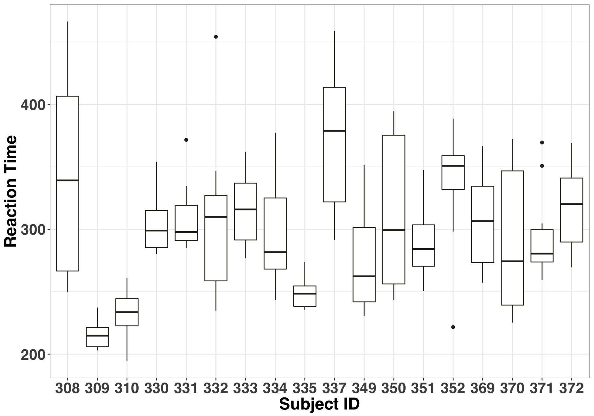
If the median of each of our boxplots were approximately equal, then we could use a fixed effect or simply not including the subject effect at all. But clearly this isn’t the case. Accordingly, here is the form of our model:
y_var = "reaction"
fixed_effect = "days"
random_effect = "subject"
model_form = as.formula(paste0(y_var, " ~ ", fixed_effect, " + ", "(1|", random_effect, ")"))
print(model_form)
## reaction ~ days + (1 | subject)Next let’s fit the model to the complete dataset and determine the experimental power based on 100 simulations using the simr package.
set.seed(1)
sleep_fit = lmer(model_form,
                 data = sleep_df)
nsim = 100
expected_power = powerSim(sleep_fit, nsim = nsim)
print(expected_power)
## Power for predictor 'days', (95% confidence interval):
## 100.0% (96.38, 100.0)
##
## Test: Kenward Roger (package pbkrtest)
## Effect size for days is 10.
##
## Based on 100 simulations, (0 warnings, 0 errors)
## alpha = 0.05, nrow = 180
##
## Time elapsed: 0 h 0 m 26 s
##
## nb: result might be an observed power calculationThis indicates that we are all but guaranteed to detect an effect if we run the study with 18 participants for a period of 10 days. The folks who did this study obviously wanted to leave nothing to chance! What if we tried to replicate the study with the same number of participants but for fewer days? How would our power change if we only ran the study for, say, three days? We’ll filter the data to only include days 0-3, and then repeat the power estimate.
set.seed(321)
n_days_max = 3
min_days_df = sleep_df %>%
              filter(days <= n_days_max)
min_days_fit = lmer(model_form, min_days_df)
expected_power = powerSim(min_days_fit, nsim = nsim)
print(expected_power)
## Power for predictor 'days', (95% confidence interval):
## 98.00% (92.96, 99.76)
##
## Test: Kenward Roger (package pbkrtest)
## Effect size for days is 4.4.
##
## Based on 100 simulations, (0 warnings, 0 errors)
## alpha = 0.05, nrow = 72
##
## Time elapsed: 0 h 0 m 18 s
##
## nb: result might be an observed power calculationReducing the number of days from 10 to three had almost no effect on our power, which is estimated to be 98%. Thus, the recommendation here would be to run the study for fewer days. Great! That was easy. Indeed, I was excited after using the simr package because of its ability to fit many different model specifications. The only issue was that I wasn’t entirely clear on the underlying process being used to calculate power. According the tutorial from the authors (see here), there are three steps involved in calculating power for mixed effects models via simulation:
- Simulate new values for the response variable using the model provided
- Refit the model to the simulated response
- Apply a statistical test to the model
It was that first part where I wasn’t entirly clear, so I decided to build my own from scratch and compare the results.
Building a Power Simulator
We established our model above as reaction ~ days + (1|subject). So what do they mean by “simulate new values for the response variable”? The new values are produced by our model plus error associated with sampling. That second part is thing we are going to simulate. We will assume the residuals are normally distributed, with a mean of zero and a standard deviation of…and a standard deviation of…aww shoot how do we come up with this number? We can initially start with the residuals from our model and use that as the standard deviation. Let’s see if we can produce a result similiar to the 98% estimate observed with the simr package.
set.seed(321)

# create empty vector to store Type II errors
type_II_vec = c()
# Step 1: make predictions from  model based on the original data
model_predictions = predict(min_days_fit, min_days_df)
# Step 2: Calculate  standard deviation based on the residuals from our initial model
standard_deviation = sd(min_days_fit@resp$y - min_days_fit@resp$mu)

for(i in 1:nsim){
  # Step 3: Simulate  sampling error
  temporary_residuals = rnorm(nrow(min_days_df),
                              mean = 0,
                              sd = standard_deviation)
  # Step 4: Save simulated response values
  min_days_df$simulated_reaction = model_predictions + temporary_residuals
  # Step 5: refit the model with the new, simulated response variable
  temp_fit = lmer(simulated_reaction ~ days + (1|subject), data = min_days_df)
  # Step 6: Check to see if confidence interval for the Days coefficient contains zero
  ci_df = tidy(confint(temp_fit)) %>%
              dplyr::rename(coefficients = .rownames,
              lower_bound = X2.5..,
              upper_bound = X97.5..) %>%
          filter(coefficients == 'days') %>%
          dplyr::select(lower_bound, upper_bound)
  # Step 7: If Confidence interval contains zero, store as 1 (Type II error), else return store zero
  type_II_vec = c(type_II_vec,
                  as.integer(dplyr::between(0, ci_df$lower_bound, ci_df$upper_bound)))
}
print(paste0("EXPECTED POWER IS: ", (nsim - sum(type_II_vec))/nsim * 100, "%"))
## [1] "EXPECTED POWER IS: 99%"Exactly what we expected. Of our 100 simulations, we commited a type II error in only one instance, which matches closely with the 98% estimate provided from the simr package. If we increased the number of simulations, the power estimates would converge to the same number. However, if you copied this code and ran it in R, you’ll notice that it ran slow. In a separate post, I’ll show you how to speed up any simulation by executing the entire process in parallel to run more simulations and get better estimates! Stay tuned!