Overview
There are few reasons for reducing the number of potential input features when building a model:
- Faster training times
- Easier interpretation
- Improved accuracy by reducing the chance of overfitting
The focus here will primarly be on point three, as we address two questions:
- Does having noisy, unnecessary variables as inputs reduce classification performance?
- And, if so, which algorithms are the most robust to the ill-effects of these unnecessary variables?
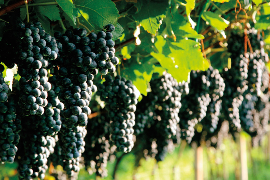
We’ll explore these questions with one my favorite datasets located here. Based on the methodology outlined here, a bunch of Wine experts got together and evaluated both White and Red wines. Each row represents the chemical properties of a wine in addition to a rating (0 = very bad, 10 = excellent). Each wine was rated by at least three people, and the median of their ratings was used as the final score. I have no idea how you get paid to drink wine, but somewhere in my life, I chose the wrong career path. Thus, the goal here is to predict the rating based on the chemical properties of the wine, such as its pH or Alcohol Concentration.
Let’s load up the libraries we’ll need as well as a custom plotting function.
Here we’ll read the wine quality ratings directly for the source. We’ll also convert the rating system from a 1-10 scale to binary for the sake of simplicity. Any wine with a rating greater than seven receives the highly coveted “IdDrinkThat”, while all others receive the dreaded “NoThanks” label.
red_file = 'winequality-red.csv'
white_file = 'winequality-white.csv'
base_url = 'https://archive.ics.uci.edu/ml/machine-learning-databases/wine-quality/'
red_wine = fread(paste0(base_url, red_file)) %>%
           data.frame()
white_wine = fread(paste0(base_url, white_file)) %>%
           data.frame()
wine_df = bind_rows(red_wine,
                    white_wine
                    ) %>%
          clean_names() %>%
          mutate(wine_class = ifelse(quality >= 7,
                                            "IdDrinkThat",
                                            "NoThanks")) %>%
          mutate(wine_class = as.factor(wine_class)) %>%
          select(-quality)
As usual, let’s peak at the data to make sure there aren’t any unwanted surprises.
| fixed_acidity | volatile_acidity | citric_acid | residual_sugar | chlorides | free_sulfur_dioxide | total_sulfur_dioxide | density | ph | sulphates | alcohol | wine_class |
|---|---|---|---|---|---|---|---|---|---|---|---|
| 7.4 | 0.700 | 0.00 | 1.9 | 0.076 | 11 | 34 | 0.9978 | 3.51 | 0.56 | 9.4 | NoThanks |
| 7.8 | 0.880 | 0.00 | 2.6 | 0.098 | 25 | 67 | 0.9968 | 3.20 | 0.68 | 9.8 | NoThanks |
| 7.8 | 0.760 | 0.04 | 2.3 | 0.092 | 15 | 54 | 0.9970 | 3.26 | 0.65 | 9.8 | NoThanks |
| 11.2 | 0.280 | 0.56 | 1.9 | 0.075 | 17 | 60 | 0.9980 | 3.16 | 0.58 | 9.8 | NoThanks |
| 7.4 | 0.700 | 0.00 | 1.9 | 0.076 | 11 | 34 | 0.9978 | 3.51 | 0.56 | 9.4 | NoThanks |
| 7.4 | 0.660 | 0.00 | 1.8 | 0.075 | 13 | 40 | 0.9978 | 3.51 | 0.56 | 9.4 | NoThanks |
| 7.9 | 0.600 | 0.06 | 1.6 | 0.069 | 15 | 59 | 0.9964 | 3.30 | 0.46 | 9.4 | NoThanks |
| 7.3 | 0.650 | 0.00 | 1.2 | 0.065 | 15 | 21 | 0.9946 | 3.39 | 0.47 | 10.0 | IdDrinkThat |
| 7.8 | 0.580 | 0.02 | 2.0 | 0.073 | 9 | 18 | 0.9968 | 3.36 | 0.57 | 9.5 | IdDrinkThat |
| 7.5 | 0.500 | 0.36 | 6.1 | 0.071 | 17 | 102 | 0.9978 | 3.35 | 0.80 | 10.5 | NoThanks |
| 6.7 | 0.580 | 0.08 | 1.8 | 0.097 | 15 | 65 | 0.9959 | 3.28 | 0.54 | 9.2 | NoThanks |
| 7.5 | 0.500 | 0.36 | 6.1 | 0.071 | 17 | 102 | 0.9978 | 3.35 | 0.80 | 10.5 | NoThanks |
| 5.6 | 0.615 | 0.00 | 1.6 | 0.089 | 16 | 59 | 0.9943 | 3.58 | 0.52 | 9.9 | NoThanks |
| 7.8 | 0.610 | 0.29 | 1.6 | 0.114 | 9 | 29 | 0.9974 | 3.26 | 1.56 | 9.1 | NoThanks |
| 8.9 | 0.620 | 0.18 | 3.8 | 0.176 | 52 | 145 | 0.9986 | 3.16 | 0.88 | 9.2 | NoThanks |
| 8.9 | 0.620 | 0.19 | 3.9 | 0.170 | 51 | 148 | 0.9986 | 3.17 | 0.93 | 9.2 | NoThanks |
| 8.5 | 0.280 | 0.56 | 1.8 | 0.092 | 35 | 103 | 0.9969 | 3.30 | 0.75 | 10.5 | IdDrinkThat |
| 8.1 | 0.560 | 0.28 | 1.7 | 0.368 | 16 | 56 | 0.9968 | 3.11 | 1.28 | 9.3 | NoThanks |
| 7.4 | 0.590 | 0.08 | 4.4 | 0.086 | 6 | 29 | 0.9974 | 3.38 | 0.50 | 9.0 | NoThanks |
| 7.9 | 0.320 | 0.51 | 1.8 | 0.341 | 17 | 56 | 0.9969 | 3.04 | 1.08 | 9.2 | NoThanks |
| 8.9 | 0.220 | 0.48 | 1.8 | 0.077 | 29 | 60 | 0.9968 | 3.39 | 0.53 | 9.4 | NoThanks |
| 7.6 | 0.390 | 0.31 | 2.3 | 0.082 | 23 | 71 | 0.9982 | 3.52 | 0.65 | 9.7 | NoThanks |
| 7.9 | 0.430 | 0.21 | 1.6 | 0.106 | 10 | 37 | 0.9966 | 3.17 | 0.91 | 9.5 | NoThanks |
| 8.5 | 0.490 | 0.11 | 2.3 | 0.084 | 9 | 67 | 0.9968 | 3.17 | 0.53 | 9.4 | NoThanks |
| 6.9 | 0.400 | 0.14 | 2.4 | 0.085 | 21 | 40 | 0.9968 | 3.43 | 0.63 | 9.7 | NoThanks |
This dataset is exceptionally clean. Typically we would do some exploratory analysis to check for outliers, missing values, incorrect codings, or any other number of problems that can sabotage our predictions. In this case, we can go right into the variable selection.
We’ll initially leverage the gradient boosted machine (GBM) algorithm in the h2o library for variable selection. One of the nice features of GBM is that it automatically tells you which variables are important. Recall that GBM is an iterative algorithm that fits many simple decision trees, where the errors from the prior tree become the dependent variable for each subsequent tree. A feature’s importance is determined by how much its introduction into a given tree reduces the error. The total reduction in error for a given feature is then averaged across all of the trees the feature appeared in. Thus splitting on important variables should lead to larger reductions in error during training relative to less important variables.
With that in mind let’s do an initial pass and see which variables are important. We’ll do a 70⁄30 train/test split, start h2o, and fit an initial model.
trainTestSplit = function(df, split_proportion){
  set.seed(123)
  out_list = list()
  data_split = sample(1:2,
                      size = nrow(df),
                      prob = split_proportion,
                      replace = TRUE)

  out_list$train = df[data_split == 1,]
  out_list$test = df[data_split == 2,]
  return(out_list)
}
split_proportion = c(0.7, 0.3)
df_split = trainTestSplit(wine_df, split_proportion)
Next we’ll calculate our variable importance metric.
h2o.init(nthreads = -1)
train_h2o = as.h2o(df_split$train)
test_h2o = as.h2o(df_split$test)
y_var = "wine_class"
x_var = setdiff(names(train_h2o), y_var)
gbm_fit = h2o.gbm(x = x_var,
                  y = y_var,
                  distribution = "bernoulli",
                  training_frame = train_h2o,
                  stopping_rounds = 3,
                  stopping_metric = "AUC",
                  verbose = FALSE
                  )
And let’s plot our results based on the relative importance of each feature.
  data.frame(gbm_fit@model$variable_importances) %>%
    select(variable, relative_importance) %>%
    mutate(relative_importance = round(relative_importance),
                variable = factor(variable)) %>%
    mutate(variable = fct_reorder(variable,
                                  relative_importance, .desc = TRUE)) %>%
  ggplot(aes(x = variable,
             y = relative_importance,
             fill = variable,
             label = as.character(relative_importance))) +
    geom_bar(stat = "identity") +
    geom_label(label.size = 1, size = 5, color = "white")  +
    theme_bw() +
    my_plot_theme() +
    theme(legend.position = "none") +
    ylab("Relative Importance") +
    xlab("Variable") +
    theme(axis.text.x = element_text(angle = 90, hjust = 1, size = 12))
It looks like all of the variables have some degree of influence on classification, so we’ll continue with the full model. Next, we’re going to calculate AUC (Area Under Curve) for the following methods:
- GBM
- Random Forest (RF)
- Neural Network (NN)
- Logistic Regression (LR)
We’ll use this as a point of comparison as additional irrelevant predictor variables are added. Our goal is to see how the addition of such variables affects AUC on the test set. Let’s calculate our baseline numbers.
rf_fit = h2o.randomForest(x = x_var,
                          y = y_var,
                          training_frame = train_h2o,
                          stopping_rounds = 3,
                          stopping_metric = "AUC"
                          )

nn_fit = h2o.deeplearning(x = x_var,
                          y = y_var,
                          training_frame = train_h2o,
                          stopping_rounds = 3,
                          stopping_metric = "AUC")

glm_fit = h2o.glm(x = x_var,
                   y = y_var,
                   family = "binomial",
                   training_frame = train_h2o)

gbm_auc = h2o.auc(h2o.performance(gbm_fit, newdata = test_h2o))
rf_auc = h2o.auc(h2o.performance(rf_fit, newdata = test_h2o))
nn_auc = h2o.auc(h2o.performance(nn_fit, newdata = test_h2o))
glm_auc = h2o.auc(h2o.performance(glm_fit, newdata = test_h2o))

auc_df = data.frame(n_noise_vars = rep(0, 4),
                    method = c('gbm', 'rf', 'nn', 'glm'),
                    AUC = c(gbm_auc, rf_auc, nn_auc, glm_auc)) %>%
arrange(desc(AUC))| n_noise_vars | method | AUC |
|---|---|---|
| 0 | rf | 0.9186806 |
| 0 | gbm | 0.8889589 |
| 0 | nn | 0.8417844 |
| 0 | glm | 0.8179276 |
This provides us with a general baseline. In the following section, we’ll see what happens to the Area Under the Curve (AUC) as we add in lots of irrelevant predictors. But first, let’s explore why we are using AUC as our evaluation metric.
AUC as a Measure of Classification Accuracy
Measuring model performance when your dependent variable is binary is more “involved” than measuring performance with a continuous dependent variable. With a continuous DV, large residuals are worse than small residuals, and this can be quantified along a continuum. In contrast, you can have a classifier that’s extremely accurate – it provides the correct classification 99.99% of the time – but actually doesn’t tell you anything useful. This situation typically arises when you have imbalanced classes, such as trying to predict whether or not someone has a disease when it only occurs in 1 of 100,000 people. By chance alone, the classifier would be right 99,999 times out of 100,000 if you just said: “no one has the disease ever”.
Let’s consider the class balance in our wine dataset
print(round(table(wine_df$wine_class)/nrow(wine_df) * 100, 1))##
## IdDrinkThat NoThanks
## 19.7 80.3According to our refined, discerning pallette, 80% of wines would fall by chance alone in the “NoThanks”" category. We could achieve 80% accuracy by simply assigning a label of “NoThanks” to every new wine we encountered. This would obviously be a terrible idea, because then we’d never get to drink any wine! Thus, in cases where your classes are unevenly distributed, accuracy might not be the best evaluation metric.
AUC isn’t affected by class imbalances because it considers both True Positives and False Positives. The True Positive Rate (TPR) captures all the instances in which our model said ‘Drink this wine’ and it was, in fact, a wine we would want to drink; False Positive Rate (FPR) captures instances in which our model said ‘Drink this Wine’ but it was actually a wine that we would not want to drink. Obtaining more TPRs and fewer FPRs will move the AUC closer to one, which means our model is improving. Hopefully, this clarifies the rationale for using AUC relative to accuracy. Now let’s get back to the original question.
Adding Irrelevant Predictors
A little disclaimer before moving on. There are a number of ways you can reduce the influence of irrelevant features on predictive accuracy, namely regularization. However, we’re interested in which algorithms are least susceptible to modeling the noise associated with an irrelevant predictor variable without any additional regularization or parameter optimization. Accordingly, we’ll sample the irrelevant predictors from a normal distribution with a mean of zero and a standard deviation of one. Each iteration adds an additional 100 irrelevant predictors across a total of 20 iterations. All of the algorithms use the default parameters that come with the h2o library.
n_noise_vars = seq(100, 2000, length.out = 20)

for(i in n_noise_vars){
  print(i)
  temp_noise_df_train = data.frame(placeholder = rep(NA, nrow(df_split$train)))
  temp_noise_df_test = data.frame(placeholder = rep(NA, nrow(df_split$test)))

  # add in i irrelevant predictors to train and test
  for(j in 1:i){
    temp_noise_df_train = cbind(temp_noise_df_train,
                                data.frame(noise.var = rnorm(nrow(df_split$train),
                                                           0,
                                                           1)))
    temp_noise_df_test = cbind(temp_noise_df_test,
                               data.frame(noise.var = rnorm(nrow(df_split$test),
                                                           0,
                                                           1)))
  }
  # format names of irrelevant variables
  temp_noise_df_train = temp_noise_df_train[,2:dim(temp_noise_df_train)[2]]
  names(temp_noise_df_train) = gsub("\\.", "", names(temp_noise_df_train))
  temp_noise_df_train = as.h2o(cbind(temp_noise_df_train,
                              df_split$train))

  temp_noise_df_test = temp_noise_df_test[,2:dim(temp_noise_df_test)[2]]
  names(temp_noise_df_test) = gsub("\\.", "", names(temp_noise_df_test))
  temp_noise_df_test = cbind(temp_noise_df_test,
                             df_split$test)

  x_var = setdiff(names(temp_noise_df_train),y_var)

  gbm_fit = h2o.gbm(x = x_var,
                    y = y_var,
                    distribution = "bernoulli",
                    training_frame = temp_noise_df_train,
                    stopping_rounds = 3,
                    stopping_metric = "AUC")

  rf_fit = h2o.randomForest(x = x_var,
                            y = y_var,
                            training_frame = temp_noise_df_train,
                            stopping_rounds = 3,
                            stopping_metric = "AUC")

  nn_fit = h2o.deeplearning(x = x_var,
                            y = y_var,
                            training_frame = temp_noise_df_train,
                            stopping_rounds = 3,
                            stopping_metric = "AUC")

  glm_fit = h2o.glm(x = x_var,
                    y = y_var,
                    family = "binomial",
                    training_frame = temp_noise_df_train)

  temp_noise_df_test = as.h2o(temp_noise_df_test)

  gbm_auc = h2o.auc(h2o.performance(gbm_fit, newdata = temp_noise_df_test))
  rf_auc = h2o.auc(h2o.performance(rf_fit, newdata = temp_noise_df_test))
  nn_auc = h2o.auc(h2o.performance(nn_fit, newdata = temp_noise_df_test))
  glm_auc = h2o.auc(h2o.performance(glm_fit, newdata = temp_noise_df_test))

  auc_df = rbind(auc_df,
                 data.frame(n_noise_vars = i,
                 method = c('gbm', 'rf', 'nn', 'glm'),
                 AUC = c(gbm_auc, rf_auc, nn_auc, glm_auc)))
}
And now let’s plot the results.
ggplot(auc_df, aes(x = n_noise_vars,
                   y = AUC,
                   color = method)) +
         geom_point(size = 2) +
  stat_smooth(span = 1.75,
              se = FALSE,
              size = 2) +
  theme_bw() +
  my_plot_theme() +
  ylab("AUC") +
  xlab("N Noise Variables")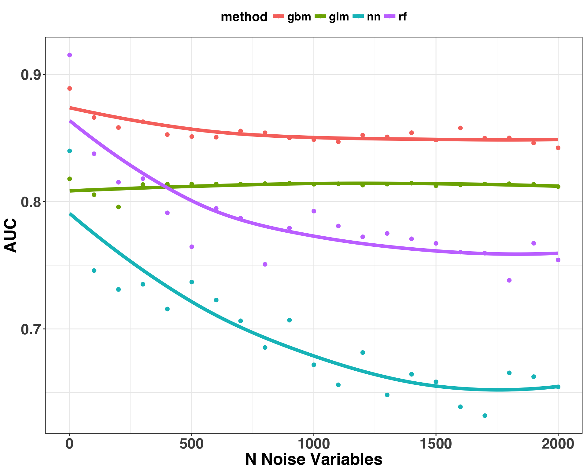
A few initial observations:
- AUC for all methods, with the exception of GLM, decreased as the number of irrelevant predictors in the model increased
- GBM is the most robust against the ill-effects of irrelevant predictors, while NN was the most susceptible
Although we can’t generalize these outcomes to every situation, they do align with my experience. In fact, one of the reasons I like GBM is that it tends to ignore irrelevant predictors during modeling. Neural networks are extremely powerful and with the right tuning/regularization will often outperform any of the methods outlined here. However, they are susceptible to overfitting because of their flexibility, which leads to noise being leveraged as signal during the model building process. This goes to show that pre-processing and feature selection is an important part of the model building process if you are dealing with lots of potential features. Beyond reducing the training time, pruning irrelevant features can vastly improve model performance. As illustrated above, including irrelevant features can wreak havoc on your model when using methods with lots of flexible parameters. It would be interesting to see how these results change if we added some regularization measures to protect against overfitting. For example, one way to reduce overfitting with Random Forest is to limit the maximum depth of a tree (i.e., each tree can only have a single split instead of multiple splits). Or for Neural Networks L2 regularization can be used, which discourages weight vectors in the network from becoming too large. If you try any of these approaches, I’d love to hear how it goes!